This article documents my thoughts and processes on my first Kaggle competition. The objective of this competition was to identify salt from sub-surface geological images. Professional seismic imaging still requires expert human interpretation of salt bodies, leading to subjective, highly variable renderings. The variability in these results can lead to potentially dangerous scenarios for oil and gas drilling companies. The competition was posted in an attempt to garner machine-learning based solutions that could improve the status-quo.
Given that this was my first competition and that I would only be able to work on the competition in my spare time, my objectives were to get a feel for how the competition process worked, apply my skills to an interestng and different problem, and to work on developing new skills and knowledge. With that covered, let’s dive in!
Model Selection
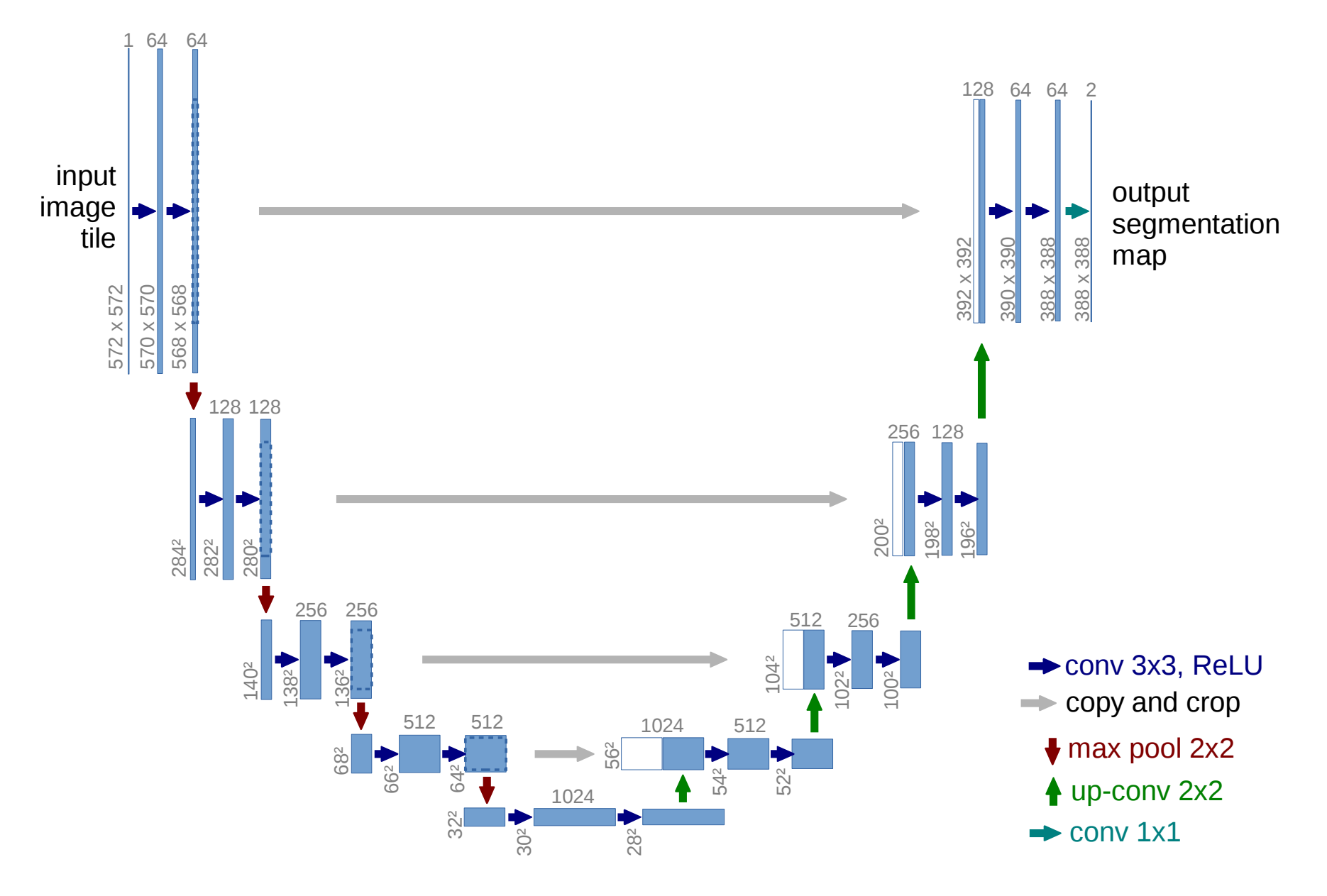
For this challenge, I chose to build a U-net model, as their ability to perform image segmentation suits the given challenge. At a high level, U-nets are a convolutional neural network model where for each layer, the X and Y dimensions slowly decrease and the number of filters (Z dimension) increases relative to the previous layer. Once this process has happened a few times (the extent of this decreasing is a model hyper-parameter), the opposite then happens, with layer X and Y dimensions increasing as the number of filters decreases. Finally, there is a layer at the end for per-pixel classification based on the segmentation. An image of an example u-net (from the linked paper) encapsulating this process is shown below.
Data Loading and Segmentation
I used the python package pandas to import the data. A separate data frame was used for the training and test data. Each of the data frames contained image identifiers, the depth the image was taken, and the actual image itself. The code snippet for generating these data frames is below.
train_df = pd.read_csv("./train.csv", index_col="id", usecols=[0])
depths_df = pd.read_csv("./depths.csv", index_col="id")
train_df = train_df.join(depths_df)
test_df = depths_df[~depths_df.index.isin(train_df.index)]

print('Loading Training Images...')
train_df["images"] = [np.array(load_img(train_image_dir+"{}.png".format(idx), grayscale=True)) / 255
                      for idx in tqdm_notebook(train_df.index)]
print('Loading Training Masks...')
train_df["masks"] = [np.array(load_img(train_mask_dir+"{}.png".format(idx), grayscale=True)) / 255
                     for idx in tqdm_notebook(train_df.index)]
To learn optimal model parameters, it is necessary to split the training data into two sets, model training and model validation. In particular, the final layer of the model will be a sigmoid layer, and the validation data will be used here to set an optimal threshold value for classification of each pixel as either salt or not salt.
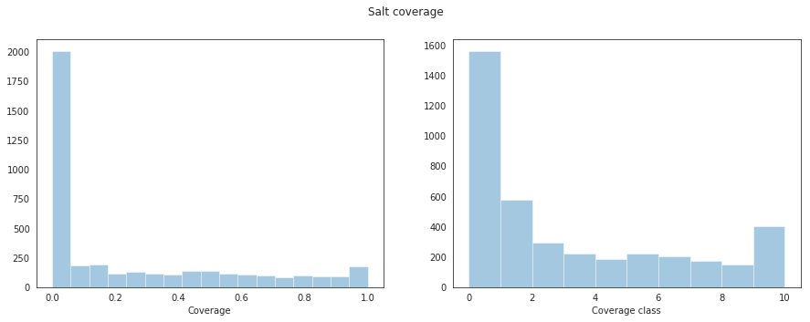
In addition to this, the data in the training and the validation sets need to be similar (and ideally the test data set too). In a simplistic sense, this is required so that we can compare ‘apples to apples’. To achieve this similarity in the salt training data set, I gave each image a label from 0-10 based on the amount of salt present (this information is in the training labels). The salt coverage in each training image and the corresponding classification label were added to the training data frame as shown below.
train_df["coverage"] = train_df.masks.map(np.sum) / pow(img_size_orig, 2)

def cov_to_class(val):
    for i in range(0, 11):
        if val * 10 <= i :
            return i

train_df["coverage_class"] = train_df.coverage.map(cov_to_class)
Looking at the salt coverage and the corresponding classification labels across the training images we get the following result.
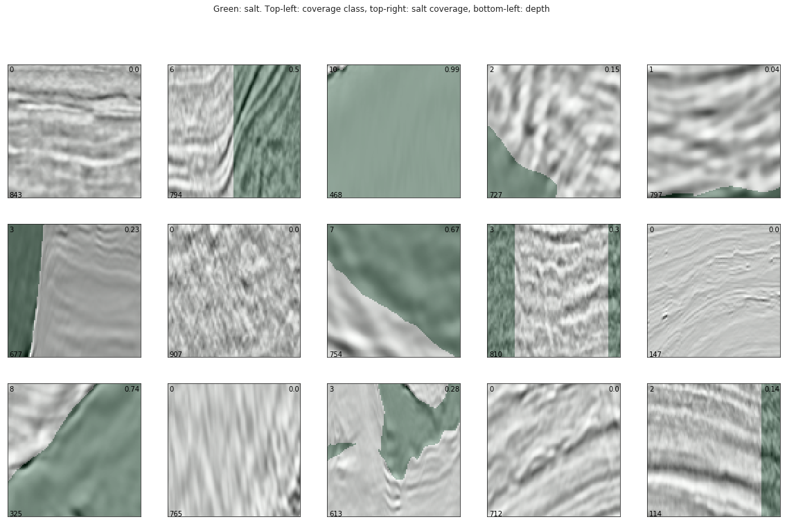
And below we can see a handful of example salt images with the salt location labels overlayed in green. The coverage class (top-left), amount of salt present (top-right), and depth the image was taken (bottom-left) are shown on each of the example images. Looking at these images, we can see that in some cases the salt coverage doesn’t align with the corresponding image. This is a peculiarity that warrants further investigation at a later stage (note that I didn’t get to look at this due to time reasons).
Now that each image has a classification label based on its salt content, the images can now be split into subsets. The requirement when assigning the images to each subset is that each subset has the same number of images per classification label. This is to maintain the similarity mentioned earlier. To split the images, I used the StratifiedKFold function from the scikit-learn package, and split the data into 5 subsets. The code snippet below shows this (validation_size=5). It should be noted that the number of subsets to generate is a hyper-parameter of the overall model, and as such it could be worth looking into other potential values.
train_df['validation_iter'] = 0

#http://scikit-learn.org/stable/modules/generated/sklearn.model_selection.StratifiedKFold.html
skf = StratifiedKFold(n_splits=validation_size, shuffle=True, random_state = 45)
for i, (train_index, test_index) in enumerate(skf.split(train_df.images, train_df.coverage_class)):
    X_test = train_df.coverage_class[test_index]
    train_df.loc[X_test.index, 'validation_iter'] = i
Finally, for a quick sanity check, we look at the number of samples per subset as well as the distribution of the classification labels in each subset. From the code snippets below, we can see that the data has been segmented as required.
sum_validations = 0
for count in range(0,validation_size):
    num_validation_data = len(train_df.loc[train_df.validation_iter == count ])
    print('For validation set ' + str(count) + ' there were ' + str(num_validation_data) + ' samples')
    sum_validations += num_validation_data

print('In total, there were ' + str(sum_validations) + ' samples')

    For validation set 0 there were 804 samples
    For validation set 1 there were 801 samples
    For validation set 2 there were 800 samples
    For validation set 3 there were 799 samples
    For validation set 4 there were 796 samples
    In total, there were 4000 samples
num_row = validation_size
num_col = 11
valid_set = [[0] * num_col for i in range(num_row)]
for count in range(0,validation_size):
for salt_class in range(0,11):
valid_set[count][salt_class] = len(train_df.loc[(train_df.validation_iter == count) &
(train_df.coverage_class == salt_class)])
print('Rows represent each validation set.')
print('Columns represent each classification label.')
valid_set
Rows represent each validation set.
Columns represent each classification label.
[[313, 116, 60, 45, 38, 45, 41, 35, 30, 32, 49],
[313, 115, 59, 45, 37, 45, 41, 35, 30, 32, 49],
[312, 115, 59, 45, 37, 45, 41, 35, 30, 32, 49],
[312, 115, 59, 45, 37, 45, 41, 35, 29, 32, 49],
[312, 115, 59, 44, 37, 45, 41, 34, 29, 31, 49]]Before moving on, another (and potentially better) way to organise the data would be via depth. One of the major advantages of using depth is that it is information that is also available from the test data set. This would provide a way to ensure some measure of similarity between the training subsets and the test data set. Dividing the data this way (or even include the depth data) was not something I looked at. This idea came from one of the top competitor results whose model was similar to mine.
Data Augmentation
Data augmentation can be a useful method of increasing the amount of training data available. The idea is to take the training data you currently have and then modify it in a ‘reasonable’ way to produce more training data. What constitutes reasonable is dependent on the problem that one is trying to solve. In this problem, I looked into augmenting the training data in a few ways: flipping each image along the horizontal axis, flipping each image along the vertical axis, rotating the image (90,189,270 degrees), and a combination of the listed transformations.
The validity of these augmentation methods ultimately depends on whether they improve the model. As such, it is worth looking at all reasonable methods of data augmentation.
Model Definition
To assist with the building of the model, I define two similar functions, one for building the steps down the model, and the other for building the steps up the model. These functions will allow for cleaner model construction code. Again here, there are several hyper-parameters that will influence the structure of the model. Some examples include the number of convolution layers per step and the dilation rate of the convolutional layers (a parameter that effects the ‘spread’ of the convolutional pixels). The snippet below shows the definition for each of these functions.
def down_layer(input_layer, num_conv, num_features, dil_rate):

    output_layer = MaxPooling2D(2)(input_layer)
    output_layer = Dropout(0.2)(output_layer)

    output_layer = Conv2D(num_features, 3, activation='relu', padding='same')(output_layer)
    for count in range(0,num_conv-1):
        output_layer = Conv2D(num_features, 3, activation='relu', padding='same', dilation_rate=dil_rate)(output_layer)

    return output_layer

def up_layer(input_layer, concat_layer, num_conv, num_features):

    output_layer = Conv2DTranspose(num_features, 3, strides=2, padding="same")(input_layer)
    output_layer = Dropout(0.4)(output_layer)
    output_layer = concatenate([concat_layer, output_layer])

    for count in range(0,num_conv):
        output_layer = Conv2D(num_features, 3, activation='relu', padding='same')(output_layer)

    return output_layer
With the functions above, the model can now be constructed and the snippet for this is shown below. The model assembly process is relatively straightforward. First an input layer of a specific shape is defined, and is where the images will be loaded into the model. I have chosen a layer of size 128*128 (the images are 101*101, so some padding will be required). Having image dimensions as a multiple of 2 allows for the potential of more ‘depth’ in the u-net model, as the dimensions are halved at each step down. Again, the size of the input image and the scaling of the original image are design choices that will influence the performance of the model.
With the initial layer defined, the ‘step-down’ and ‘step-up’ sections of the model are constructed by calling the previously defined functions. These stages are defined in a loop that controls how ‘deep’ the model is. Finally, a sigmoid layer is added to the end to perform the segmentation, and the model is defined from the constructed layers. The use of jump_stack in the snippet below is to construct the connections from the down-steps to the up-steps (gray lines in the first image that describes the u-net).
    #Initialise list of Unet jump paths
    jump_stack = []

    input_layer = Input(shape=(128,128,1))

    #Build initial Unet layer
    curr_layer = Conv2D(start_conv_val * 1, (3, 3), activation="relu", padding="same")(input_layer)
    for i in range(0,conv_tier_val-1):
        curr_layer = Conv2D(start_conv_val * 1, (3, 3), activation="relu", padding="same")(curr_layer)
    jump_stack.append(curr_layer)

    #Build down path of Unet
    for i in range(0,sub_depth_val):
        curr_layer = down_layer(curr_layer, conv_tier_val, start_conv_val*2**(i+1), dilate_val)
        jump_stack.append(curr_layer)

    jump_stack.pop()
    #Build up path of Unet
    for i in range(sub_depth_val,0,-1):
        curr_layer = up_layer(curr_layer, jump_stack[-1], conv_tier_val, start_conv_val*2**(i-1))
        jump_stack.pop() #Remove the most recent jump path

    output_layer = Conv2D(1, kernel_size=1, activation='sigmoid')(curr_layer)
    model = Model(inputs = input_layer, outputs = output_layer)
Model Training and Validation
With the model now defined, it can now be compiled. Given that I am trying to perform image segmentation I chose to use a binary_crossentropy loss function, and the metric I am interested in is the accuracy of the model. To train the model, I also chose a static, small learning rate. Choosing an optimal, or even variable learning rate would be something to look into in the future. The code to set these parameters up is shown below.
    opt = keras.optimizers.Adam(lr=0.00001)
    #model.compile(loss="binary_crossentropy", optimizer="adam", metrics=["accuracy"])
    model.compile(loss="binary_crossentropy", optimizer=opt, metrics=["accuracy"])
    model_save_loc = folder_loc + '/keras.model'
    early_stopping = EarlyStopping(patience=40, verbose=0)
    model_checkpoint = ModelCheckpoint(model_save_loc, save_best_only=True, verbose=0)

    history = model.fit(x_train_padded, y_train_padded,
                validation_data=[x_val_padded, y_val_padded],
                epochs=epochs,
                batch_size=batch_size,
                callbacks=[early_stopping, model_checkpoint])
Once the model has been trained, the best performing iteration is then reloaded. The model performance metric chosen for the competition was a variant of intersection over union metric. This metric takes the intersection of the segmentation label pixels with the model prediction pixels and then divides it by the union of the pixels from the label and prediction that contain salt. Using this metric, the thresholding value for the final segmentation layer is defined to complete the learned model (note this code is not shown here and was something that I borrowed from the Kaggle competition forums).
Now with the model trained, the test images can be passed through to obtain predictions of salt location in each of the images. As mentioned earlier, I chose to work with images of 128*128 pixels to allow for multiple u-net layers to be produced. This means that the original images needed to scaled up, and to do this I chose to pad the image with its reflection (note that this process also happens in the prior data augmentation stage for the training images as well). The code to achieve this can be seen in the snippet below.
    x_test = np.array([np.array(load_img(test_image_dir+"{}.png".format(idx), grayscale=True)) / 255
                        for idx in test_df.index])
    x_test_padded = [cv2.copyMakeBorder(x,13,14,13,14,cv2.BORDER_REFLECT)
                        for x in x_test]
    x_test_padded = np.array(x_test_padded).reshape(-1, 128, 128, 1)

    #Predict
    preds_test = model.predict(x_test_padded)
    preds_test = preds_test[:, 13:114, 13:114]
Prediction Submission and Results
Once the binary images for test predictions have been generated from the above code, they can then be codified into the appropriate representation for submission (not shown here). Through the limited time I had in trying different combinations of design hyper-parameters, my best result on the public leaderboard was an accuracy of 76.2% across all test images. This translated to an accuracy of 73% on the final graded image test set.
To get the above result, my first layer started with 16 convolutional filters (and then doubled on each down-step of the u-net), there were a total of three ‘step-down’ pieces (and consequently step-up pieces too), and there were two blocks ofconvolutional filters at each step.
A tweak that I played with a little was taking images that had a low salt pixel count (for the above model, anything less than 30 pixels), and replace the predictions with a blank no-salt prediction. This was done as the penalty for guessing wrong on zero (and to a lesser extent low) salt content images is severe. Guessing anything other than a blank on an image with no salt gives a score of 0, while correctly guessing blank gives a perfect score. This modification gave an approximate improvement of 1%.
Discussion
Overall, I was happy with my score given the circumstances under which I entered the competition. I built a ‘reasonable’ model (the winning model had a 90% accuracy) for predicting the presence of salt from seismic images from scratch, in a limited time frame, in my first Kaggle competition. I met my objective of learning a lot over a relatively short time in working through this competition, and it was nice to see community discussion and idea exploration in an area that I was interested in. Through review and comparison of some of the high performing models, I was definitely on the right track with my implementation, I just needed to invest a little more.
There were several ideas that occured during (and after) the project that I would like to look at incorporating into models for future competitions. Some of these ideas included:
- Cyclical Learning Rates +The idea here is to have a decreasing learning rate to focus on a local minima when optimising, and then have a sudden spike, or increase in the learning rate to try and force the model into a new local minima, allowing for a more thorough search of the hyper-parameter space.
- Investigation into different loss functions. Some options include:
- Jaccard
- Dice
- Mean IoU
- Build an ensemble of different models.
- In my work, I split the training data in a 1:4 ratio of train:validate. I could have done this 4 more times (using a different training set each time) and then taken the average of all the results. This should lead to a more robust model overall.
- Explore more data augmentation strategies. One option that others tried was to double the size of the training images, and then randomly sampled an image of the original size from the imflated image. More ‘sensible’ data augmenation should ideally allow for a better model to be generated.
- Look at input image sizes other than 128*128 pixels.
One thing that I found difficult in this competition (particularly as I invested more effort into it), was modification of the code to test new ideas/features. There were several design hyper-parameters that presented themselves over the course of the competition, and incorporating new ideas or exploring all permutations of included ideas in a strctured and methodical way proved challenging. Part of the challenge in this stemmed from the inital use of a Jupyter notebook, which was fantastic for ideation, and then not migrating to a more robust project environment as the project grew (Yay sunken cost fallacy!).
As a consequence of this, I spent a lot of my time looking at methods that might be more suitable to handle this, rather than working on the competition itself. An interesting tool that I came across was Pachyderm, a tool for the management of multi-stage data pipelines (DVC is another option). The idea with these tools would be to set up a data processing pipeline, while keeping the project as modular as possible. This would allow for easy implementation of new ideas, there would be minimal refactoring or rerunning of code, allowing for a more thorough and cleaner method for model generation. This is definitely something that I want to implement in a similar future competition.
I would like to close out this article with a general thanks to the Kaggle community and in particular those that took part in this competition. Without this community, there would have been no competition, no forum for discussion of ideas focused on a particular topic, and I would not have been able to learn new skills and apply myself to different challenges.